Remote Sensing
Since the mid-1950s, total stratospheric ozone amounts have been regularly measured. In the early part of this period, all measurements were made in situ from instruments released from the ground. Beginning in 1979, remote sensing by satellite began.

The first remote measurements made in the vicinity of Antarctica showed extremely low ozone levels. They were so low, in fact, that after being compared to erroneous ground-based measurements, they were not believed. From 1979 until today, a steady decrease in stratospheric ozone has been noted. The decrease has been especially obvious over Antarctica where an "ozone hole" appears in the spring, and disappears in the summer. Each year, this springtime hole covers a larger area than it had the previous year.

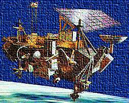
Since 1979, several satellites have been equipped with sensors that collect data on ozone, as well as other atmospheric constituents that affect the amounts of ozone present. American, Russian, and Japanese satellites have carried ozone sensors. The satellites that have flown the Total Ozone Mapping Spectrometer (TOMS) have included Meteor-3, Nimbus-7, and most recently ADEOS, and Earth Probe. The Cryogenic Limb Array Etalon Spectrometer (CLAES) is an instrument that has flown on the Upper Atmosphere Research Satellite (UARS) since 1991. The TIROS-N Operational Vertical Sounder (TOVS) measures radiances. Since all these satellites are polar orbiters, there may be gaps in data on any given day.

TOMS
A TOMS instrument was carried aboard Nimbus-7. From November 1, 1978 to May 6, 1993, this was the only source of high-resolution global information about ozone. Meteor-3, a Russian satellite, also carried a TOMS. It stopped operating on December 27, 1994. From that date until September 12, 1996, no TOMS data were available. Since then, however, the Earth Probe TOMS and ADEOS TOMS have provided data.

TOMS measures the total solar radiance incident on the satellite and, by comparing it to the uv radiation scattered back from the atmosphere, is able to compute total ozone amounts. Because it depends upon scattered solar radiation, TOMS does not work at night. As a result, between the first day of fall and the first day of spring, there will be parts of the high latitudes that will have no data. This area begins at the pole on the first day of fall, reaches its maximum on the first day of winter, and then shrinks back to zero on the first day of spring. Ozone measurements given by TOMS are in Dobson units and give the total ozone in a column. For more information about TOMS, visit the TOMS Home Page.

CLAES
The CLAES instrument was launched on UARS in 1991. Instead of measuring reflected radiation by using spectroscopy, it determines the amount of ozone by measuring the radiance emitted at several wavelengths. CLAES also measures concentrations of other substances important in ozone destruction, such as N₂O, CFCl₃(CFC-11), CF₂Cl₂(CFC-12), NO, NO₂, HNO₃, and ClONO₃.

Unlike data from TOMS, CLAES can provide data at night, since it measures emitted radiation rather than solar radiance. However, its orbit prevents collection of data in the vicinity of the poles. Unlike TOMS, CLAES data are in the form of mixing ratios at specific altitudes. For more information on CLAES, visit the Lockheed Martin Advanced Technology Center CLAES Data page.

TOVS
TOVS, launched in 1978, also measures emitted radiation. It has a band at 9700 nm, an important ozone-absorption band. Like the TOMS data, TOVS gives total ozone column concentrations in Dobson units, but the quality and accuracy of its data are dependent upon cloud conditions. TOVS data are best when collected under cloudless conditions. The NOAA satellite that carries TOVS is a polar orbiter that passes close enough to the poles to give continuous data. You can view an animation of the formation of the antarctic ozone hole and look at individual daily ozone concentrations. TOVS data: Courtesy of NGDC/NOAA

Remote Sensing Activities
1. These fifteen TOMS images show total October atmospheric ozone over the Southern Hemisphere for 1979 through 1994. To see how the ozone amounts have trended through the years, pick a longitude line for which data exist from the South Pole to the equator. For each of four latitudes: 80S, 60S, 30S, and the equator, make a graph. On each graph, place the calendar year on the X-axis, and ozone concentrations in Dobson Units on the Y-axis. If necessary, interpolate the values for ozone concentrations. After completing the four graphs, you should be able to evaluate the 15-year ozone concentration trends. What do you notice about the trends at each of the four points? What are the reasons for these trends?

2. This TOMS imagery from the ADEOS satellite is for the first day of spring. This eliminates the problem of being concerned about the length of daylight when computing radiation amounts. When determining the amount of uv radiation reaching the ground, ozone concentrations are not the only concern. Sun angle, path length through the atmosphere, and type and extent of cloudiness are all important.

For this activity, select a longitude line--taking into account ozone concentrations, sun angle, and path length through the atmosphere. Determine the amounts of uvb radiation you would expect to reach the ground at 30N and 60N relative to the amount of uvb radiation reaching Earth's surface at the equator. TOMS data: Courtesy of GSFC/NASA

3. CLAES imagery, which is valid for 8 days throughout the year, are shown for concentrations of ozone, chlorine nitrate ClONO₂, and nitric acid HNO₃. To see how the amounts have trended through the year, pick a longitude line for which data exist from the South Pole to the equator. Make a graph for each of four latitudes: 80S, 60S, 30S, and the equator. On each graph, plot the concentration values of the ozone, chlorine nitrate, and nitric acid throughout the course of the year.

Scale the values so that increments will appear somewhat equal. For ozone, use 0.3 ppmv; for nitric acid, 1 ppbv, and for chlorine nitrate, 0.2 ppbv. What trends do you see and what do they mean? CLAES data: Courtesy of Dr. A. E. Roche and the UARS/CLAES experiment at Lockheed Martin

HTML code by Chris Kreger
Maintained by ETE Team
Last updated April 28, 2005

Some images © 2004 www.clipart.com

Privacy Statement and Copyright © 1997-2004 by Wheeling Jesuit University/NASA-supported Classroom of the Future. All rights reserved.

Center for Educational Technologies, Circuit Board/Apple graphic logo, and COTF Classroom of the Future logo are registered trademarks of Wheeling Jesuit University.