
  |
Seasonal Vegetation Changes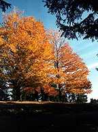 The source of the annual
cyclical variations in CO2
concentration is logically some process connected to global seasonal changes. There are
many such processes, which are natural as well as caused by humans. They include the
growth and decay of plankton in the oceans, due to annual ocean temperature changes,
seasonal changes in industrial CO2
output, due to changing heating and cooling needs, seasonal biomass burning, and the
annual growth and decay of land-based vegetation. Photo:
Courtesy of Steven K. Croft. The source of the annual
cyclical variations in CO2
concentration is logically some process connected to global seasonal changes. There are
many such processes, which are natural as well as caused by humans. They include the
growth and decay of plankton in the oceans, due to annual ocean temperature changes,
seasonal changes in industrial CO2
output, due to changing heating and cooling needs, seasonal biomass burning, and the
annual growth and decay of land-based vegetation. Photo:
Courtesy of Steven K. Croft.The challenge is to determine which process or combination of processes is responsible for the observed changes. A typical approach is (1) to carefully define the observed changes in CO2 concentration, (2) to measure the changes in CO2 due to each potential process, and (3) to compare the changes resulting from each process with the observed global changes. If both the quantity and seasonal pattern of the CO2 changes due to a particular process are similar to the quantity and pattern of the observed changes, then that process is the likely cause of the observed changes. To characterize the seasonal changes in CO2 concentration, take the monthly CO2 concentrations for the years 1992 and 1993 from the Mauna Loa data set (You will need Excel 5.0 or higher.) or the text version and enter them into a table or spreadsheet program. (The reason for selecting the 1992 and 1993 data is explained in the next paragraph.) Since only the seasonal changes are of interest here, select the smallest value of the CO2 concentration during 1992 and 1993 and subtract this value from all the others to get the differences. Graph the differences (parts per million by volume, or ppmv) as a function of time. Examine the CO2 data and record both the total amplitude of the annual changes and the times of year when maxima and minima occur. Of all the processes potentially causing the seasonal changes in CO2 concentration, biomass burning is examined in the Yellowstone Biomass Burning section, and industrial emissions is examined in the Fossil Fuel Burning section. In this section, data are presented that enable you to test the hypothesis that the seasonal CO2 changes are due to annual vegetation changes on land. The mechanism is as follows: as plants begin to grow in the spring, they absorb CO2 from the atmosphere to provide the carbon needed for new stems, roots, and leaves. As CO2 is removed from the air, atmospheric concentrations drop and will continue to drop as long as plant growth continues. As plants die and/or shed leaves in the fall, the dying plant parts decay, releasing CO2 back into the air. Atmospheric CO2 concentrations will increase as long as the decay process continues. In the spring, the cycle begins again. There are some potential problems with this process. For example, opposite seasons occur at the same time in the Northern and Southern Hemispheres. So at the same time plants are growing and absorbing CO2 during the Northern Hemisphere spring, plants are dying and releasing CO2 into the atmosphere during the Southern Hemisphere fall. If the rates of plant growth in one hemisphere are the same as the rates of plant decay in the other, they will cancel each other out and the net change in atmospheric CO2 will be zero. Similarly, seasonal biomass burning is releasing CO2 to the atmosphere during the early part of the growing season when plants in fields and forests which are not being burned are absorbing CO2. Only actual measurements of changes in global vegetation can determine how much change in atmospheric CO2 will result from this process. The main data set provided here is a set of global Normalized Difference Vegetation Index (NDVI) maps--one for each month from April 1992 to September 1993. The data were obtained from an archive maintained by the U. S. Geological Survey at the Eros Data Center in Sioux Falls, SD. The NDVI is a measure of the total amount of green vegetation per unit area on Earth's surface. Each map is a composite of the data taken the first 10 days of each month. To begin your analysis, download each map in the data set to your hard drive. Open all of the maps in NIH Image. (If you save all of the maps in a folder by themselves, you can save time by using the Open All option in the File/Open dialog box.) If you select Stacks/Windows to Stack and then Stacks/Animate, you can view the data as a movie of global vegetation changes over the course of a year. Since there are 18 months included in the complete data set, you might want to remove either the first or last six images in the stack to get a smooth one-year-long movie. Shades of yellow, orange, and light green correspond to lower DN values and denote lower vegetation density; darker shades of green correspond to higher DN values and denote higher density of vegetation. Observe the seasonal changes in your region and other regions of interest to you. In particular, contrast differences due to seasonal changes in the Northern and Southern Hemispheres. The missing data in the extreme north and south of the images at different times of the year are due to heavy clouds and lack of sunlight above the Arctic and Antarctic Circles during winter in the respective hemispheres. Once you have reviewed the geographic pattern of vegetation changes, cycle back to the beginning of the stack to begin quantitative measurements. (If you have removed some of the maps from the stack to make a year-long movie, add them back into the stack now for the quantitative analysis.) For purposes of comparison with the Mauna Loa CO2 data, you will want to measure the total global vegetation cover for each month. To do this, select Area and Integrated Density in the Analyze/Options dialog box. Activate the first map window, and use Options/Density Slice to select all of the land surfaces on the map. Then, choose Analyze/Measure and Analyze/Show Results to see the measured area (in pixels) of the land, the integrated density, and the background density. The integrated density is a measure of the total vegetative cover for that map. The background density represents the DN value for lands like the Sahara Desert that are largely barren of vegetation. Repeat the sequence for each map and export the complete data file to a table or spreadsheet. If you wish, you can find the integrated NDVI for individual continents--like your home continent--by using the freehand selection tool to outline an area of interest. Convert the global integrated NDVI to global concentration of atmospheric CO2. The actual conversion is simple, but requires some explanation. The NDVI value for each pixel is a measure of the amount of green vegetation in that pixel. If we assume a linear relation between the NDVI value, N, and the amount of vegetation visible in each pixel to the AVHRR instrument, then the mass of seasonal carbon in a pixel is about McA(N-No)/(Nmax-N0) Mc is the mass of carbon per unit area in the seasonal vegetation, A is the area of a pixel, N0 is the NDVI value for a barren desert like the Sahara, and Nmax is the NDVI value for the densest vegetation like the forests in Brazil and the Congo. The global total of seasonal carbon in each NDVI image is obtained by adding together the seasonal carbon in all of the pixels in the image. Don't be concerned, at this point: you have, in fact, already done most of the work. The integrated density, I, you just measured for each map is the sum of (N-N0) for all of the pixels in the map. So the total seasonal carbon in a map is about Total Carbon = IMcA/(Nmax-N0) Each pixel in these maps is a square 64 km on a side, so the area, A, is 4096 km2. N0 is the background value already computed when you measured the Integrated Density (Look at your Results table). You can estimate Nmax by examining the largest values in each of the maps. Good places to look are rain forests in Brazil, the Congo, and the American Northwest. Choose a typical maximum value. The final quantity, Mc, is the hardest to estimate. In the maps, you are seeing a wide variety of vegetative cover, forests, grasslands, and deserts. Estimates of carbon per unit area range from about 1 kC/m2 (kilogram of carbon per square meter) for grasslands to about 16 kC/m2 for dense forests. However, much of the carbon in forests is bound in trunks, branches, and roots, where the carbon is not released seasonally. The seasonal carbon is in leaves shed each year, annual grasses, and the stems of annual herbs. A reasonable estimate for the mass, Mc, of seasonal carbon for all types of vegetation is about 1+-0.5 kC/m2. Our best estimate is 0.6 +- 0.2 kC/m2. Find the total seasonal carbon for each map by substituting these values into the equation above and multiplying by the Integrated density, I, of each map. Then convert the seasonal carbon to seasonal CO2 for each map. As with the 1992 and 1993 CO2 data, subtract the smallest derived CO2 concentration from all of the others, and graph the result on the same graph as the Mauna Loa data. Compare the amplitude of the changes and the timing. Compare your estimates of the release of CO2 by annual biomass burning with these results for global seasonal vegetation changes. (Remember that burning of fields and forests are recorded in these NDVI data as part of the total seasonal vegetation changes.) Can global seasonal changes in vegetation account for the observed changes in atmospheric CO2 concentration?
[ Yellowstone Biomass Burning ] [ Seasonal Vegetation Changes ] [ Home ] [ Teacher Pages ] [ Modules & Activities ] |
![]()
HTML code by Chris Kreger
Maintained by ETE Team
Last updated November 10, 2004
Some images © 2004 www.clipart.com
Privacy Statement and Copyright © 1997-2004 by Wheeling Jesuit University/NASA-supported Classroom of the Future. All rights reserved.
Center for Educational Technologies, Circuit Board/Apple graphic logo, and COTF Classroom of the Future logo are registered trademarks of Wheeling Jesuit University.